Filtering Signals
In this tutorial we will practice filtering MIMIC waveform signals.
Our objectives are to:
Filter signals using the SciPy signal processing package.
Understand how to interpret the amplitude-response of a filter.
Gain experience in filtering PPG signals.
Be able to use filters to obtain the derivatives of a signal
Context: Filtering is used to eliminate noise from physiological signals. For instance, ECG signals can contain mains frequency noise due to electrical interference. Ideally, a filter would attenuate unwanted frequency content in a signal whilst retaining the physiological frequency content.
Extension: If you've not seen it before, then have a look at the SciPy signal processing package. How might it be helpful for processing PPG signals?
Setup
The following steps have been covered in previous tutorials. We’ll just re-use the previous code here.
# Packages
import sys
from pathlib import Path
!pip install wfdb==4.0.0
import wfdb
Requirement already satisfied: wfdb==4.0.0 in /Users/petercharlton/anaconda3/lib/python3.8/site-packages (4.0.0)
Requirement already satisfied: requests<3.0.0,>=2.8.1 in /Users/petercharlton/anaconda3/lib/python3.8/site-packages (from wfdb==4.0.0) (2.25.1)
Requirement already satisfied: matplotlib<4.0.0,>=3.2.2 in /Users/petercharlton/anaconda3/lib/python3.8/site-packages (from wfdb==4.0.0) (3.3.4)
Requirement already satisfied: pandas<2.0.0,>=1.0.0 in /Users/petercharlton/anaconda3/lib/python3.8/site-packages (from wfdb==4.0.0) (1.2.4)
Requirement already satisfied: scipy<2.0.0,>=1.0.0 in /Users/petercharlton/anaconda3/lib/python3.8/site-packages (from wfdb==4.0.0) (1.6.2)
Requirement already satisfied: numpy<2.0.0,>=1.10.1 in /Users/petercharlton/anaconda3/lib/python3.8/site-packages (from wfdb==4.0.0) (1.20.1)
Requirement already satisfied: SoundFile<0.12.0,>=0.10.0 in /Users/petercharlton/anaconda3/lib/python3.8/site-packages (from wfdb==4.0.0) (0.10.3.post1)
Requirement already satisfied: pillow>=6.2.0 in /Users/petercharlton/anaconda3/lib/python3.8/site-packages (from matplotlib<4.0.0,>=3.2.2->wfdb==4.0.0) (8.2.0)
Requirement already satisfied: pyparsing!=2.0.4,!=2.1.2,!=2.1.6,>=2.0.3 in /Users/petercharlton/anaconda3/lib/python3.8/site-packages (from matplotlib<4.0.0,>=3.2.2->wfdb==4.0.0) (2.4.7)
Requirement already satisfied: cycler>=0.10 in /Users/petercharlton/anaconda3/lib/python3.8/site-packages (from matplotlib<4.0.0,>=3.2.2->wfdb==4.0.0) (0.10.0)
Requirement already satisfied: kiwisolver>=1.0.1 in /Users/petercharlton/anaconda3/lib/python3.8/site-packages (from matplotlib<4.0.0,>=3.2.2->wfdb==4.0.0) (1.3.1)
Requirement already satisfied: python-dateutil>=2.1 in /Users/petercharlton/anaconda3/lib/python3.8/site-packages (from matplotlib<4.0.0,>=3.2.2->wfdb==4.0.0) (2.8.1)
Requirement already satisfied: six in /Users/petercharlton/anaconda3/lib/python3.8/site-packages (from cycler>=0.10->matplotlib<4.0.0,>=3.2.2->wfdb==4.0.0) (1.15.0)
Requirement already satisfied: pytz>=2017.3 in /Users/petercharlton/anaconda3/lib/python3.8/site-packages (from pandas<2.0.0,>=1.0.0->wfdb==4.0.0) (2021.1)
Requirement already satisfied: urllib3<1.27,>=1.21.1 in /Users/petercharlton/anaconda3/lib/python3.8/site-packages (from requests<3.0.0,>=2.8.1->wfdb==4.0.0) (1.26.4)
Requirement already satisfied: certifi>=2017.4.17 in /Users/petercharlton/anaconda3/lib/python3.8/site-packages (from requests<3.0.0,>=2.8.1->wfdb==4.0.0) (2022.12.7)
Requirement already satisfied: idna<3,>=2.5 in /Users/petercharlton/anaconda3/lib/python3.8/site-packages (from requests<3.0.0,>=2.8.1->wfdb==4.0.0) (2.10)
Requirement already satisfied: chardet<5,>=3.0.2 in /Users/petercharlton/anaconda3/lib/python3.8/site-packages (from requests<3.0.0,>=2.8.1->wfdb==4.0.0) (4.0.0)
Requirement already satisfied: cffi>=1.0 in /Users/petercharlton/anaconda3/lib/python3.8/site-packages (from SoundFile<0.12.0,>=0.10.0->wfdb==4.0.0) (1.14.5)
Requirement already satisfied: pycparser in /Users/petercharlton/anaconda3/lib/python3.8/site-packages (from cffi>=1.0->SoundFile<0.12.0,>=0.10.0->wfdb==4.0.0) (2.20)
# The name of the MIMIC IV Waveform Database on Physionet
database_name = 'mimic4wdb/0.1.0'

# Segment for analysis
segment_names = ['83404654_0005', '82924339_0007', '84248019_0005', '82439920_0004', '82800131_0002', '84304393_0001', '89464742_0001', '88958796_0004', '88995377_0001', '85230771_0004', '86643930_0004', '81250824_0005', '87706224_0003', '83058614_0005', '82803505_0017', '88574629_0001', '87867111_0012', '84560969_0001', '87562386_0001', '88685937_0001', '86120311_0001', '89866183_0014', '89068160_0002', '86380383_0001', '85078610_0008', '87702634_0007', '84686667_0002', '84802706_0002', '81811182_0004', '84421559_0005', '88221516_0007', '80057524_0005', '84209926_0018', '83959636_0010', '89989722_0016', '89225487_0007', '84391267_0001', '80889556_0002', '85250558_0011', '84567505_0005', '85814172_0007', '88884866_0005', '80497954_0012', '80666640_0014', '84939605_0004', '82141753_0018', '86874920_0014', '84505262_0010', '86288257_0001', '89699401_0001', '88537698_0013', '83958172_0001']
segment_dirs = ['mimic4wdb/0.1.0/waves/p100/p10020306/83404654', 'mimic4wdb/0.1.0/waves/p101/p10126957/82924339', 'mimic4wdb/0.1.0/waves/p102/p10209410/84248019', 'mimic4wdb/0.1.0/waves/p109/p10952189/82439920', 'mimic4wdb/0.1.0/waves/p111/p11109975/82800131', 'mimic4wdb/0.1.0/waves/p113/p11392990/84304393', 'mimic4wdb/0.1.0/waves/p121/p12168037/89464742', 'mimic4wdb/0.1.0/waves/p121/p12173569/88958796', 'mimic4wdb/0.1.0/waves/p121/p12188288/88995377', 'mimic4wdb/0.1.0/waves/p128/p12872596/85230771', 'mimic4wdb/0.1.0/waves/p129/p12933208/86643930', 'mimic4wdb/0.1.0/waves/p130/p13016481/81250824', 'mimic4wdb/0.1.0/waves/p132/p13240081/87706224', 'mimic4wdb/0.1.0/waves/p136/p13624686/83058614', 'mimic4wdb/0.1.0/waves/p137/p13791821/82803505', 'mimic4wdb/0.1.0/waves/p141/p14191565/88574629', 'mimic4wdb/0.1.0/waves/p142/p14285792/87867111', 'mimic4wdb/0.1.0/waves/p143/p14356077/84560969', 'mimic4wdb/0.1.0/waves/p143/p14363499/87562386', 'mimic4wdb/0.1.0/waves/p146/p14695840/88685937', 'mimic4wdb/0.1.0/waves/p149/p14931547/86120311', 'mimic4wdb/0.1.0/waves/p151/p15174162/89866183', 'mimic4wdb/0.1.0/waves/p153/p15312343/89068160', 'mimic4wdb/0.1.0/waves/p153/p15342703/86380383', 'mimic4wdb/0.1.0/waves/p155/p15552902/85078610', 'mimic4wdb/0.1.0/waves/p156/p15649186/87702634', 'mimic4wdb/0.1.0/waves/p158/p15857793/84686667', 'mimic4wdb/0.1.0/waves/p158/p15865327/84802706', 'mimic4wdb/0.1.0/waves/p158/p15896656/81811182', 'mimic4wdb/0.1.0/waves/p159/p15920699/84421559', 'mimic4wdb/0.1.0/waves/p160/p16034243/88221516', 'mimic4wdb/0.1.0/waves/p165/p16566444/80057524', 'mimic4wdb/0.1.0/waves/p166/p16644640/84209926', 'mimic4wdb/0.1.0/waves/p167/p16709726/83959636', 'mimic4wdb/0.1.0/waves/p167/p16715341/89989722', 'mimic4wdb/0.1.0/waves/p168/p16818396/89225487', 'mimic4wdb/0.1.0/waves/p170/p17032851/84391267', 'mimic4wdb/0.1.0/waves/p172/p17229504/80889556', 'mimic4wdb/0.1.0/waves/p173/p17301721/85250558', 'mimic4wdb/0.1.0/waves/p173/p17325001/84567505', 'mimic4wdb/0.1.0/waves/p174/p17490822/85814172', 'mimic4wdb/0.1.0/waves/p177/p17738824/88884866', 'mimic4wdb/0.1.0/waves/p177/p17744715/80497954', 'mimic4wdb/0.1.0/waves/p179/p17957832/80666640', 'mimic4wdb/0.1.0/waves/p180/p18080257/84939605', 'mimic4wdb/0.1.0/waves/p181/p18109577/82141753', 'mimic4wdb/0.1.0/waves/p183/p18324626/86874920', 'mimic4wdb/0.1.0/waves/p187/p18742074/84505262', 'mimic4wdb/0.1.0/waves/p188/p18824975/86288257', 'mimic4wdb/0.1.0/waves/p191/p19126489/89699401', 'mimic4wdb/0.1.0/waves/p193/p19313794/88537698', 'mimic4wdb/0.1.0/waves/p196/p19619764/83958172']

# Segment 0 is helpful for filtering, and 3 and 8 are helpful for differentiation
rel_segment_n = 0
rel_segment_name = segment_names[rel_segment_n]
rel_segment_dir = segment_dirs[rel_segment_n]

rel_segment_n = 8
rel_segment_name = segment_names[rel_segment_n]
rel_segment_dir = segment_dirs[rel_segment_n]
Extract one minute of noisy PPG signal from this segment
These steps have been covered in previous tutorials, so we’ll just re-use the code here.
# Specify the segment of data to be loaded
start_seconds = 20 # time since the start of the segment at which to begin extracting data
n_seconds_to_load = 60

# Load metadata for this record
segment_metadata = wfdb.rdheader(record_name=rel_segment_name, pn_dir=rel_segment_dir)
fs = round(segment_metadata.fs)
print(f"Metadata loaded from segment: {rel_segment_name}")

# Load data from this record
sampfrom = fs*start_seconds
sampto = fs*(start_seconds + n_seconds_to_load)
segment_data = wfdb.rdrecord(record_name=rel_segment_name,
                             sampfrom=sampfrom,
                             sampto=sampto,
                             pn_dir=rel_segment_dir)
print(f"{n_seconds_to_load} seconds of data extracted from: {rel_segment_name}")

# Extract the PPG signal
sig_no = segment_data.sig_name.index('Pleth')
ppg = segment_data.p_signal[:,sig_no]
fs = segment_data.fs
print(f"Extracted the PPG signal from column {sig_no} of the matrix of waveform data.")
Metadata loaded from segment: 88995377_0001
60 seconds of data extracted from: 88995377_0001
Extracted the PPG signal from column 4 of the matrix of waveform data.
Create a filter
Import the SciPy signal processing package, which contains functions for filtering and differentiating.
import scipy.signal as sp
Specify the high- and low-pass filter cut-offs
# Specify cutoff in Hertz
lpf_cutoff = 0.7
hpf_cutoff = 10
Create a Butterworth filter using the butter function
sos_ppg = sp.butter(10,
                    [lpf_cutoff, hpf_cutoff],
                    btype = 'bp',
                    analog = False,
                    output = 'sos',
                    fs = segment_data.fs)

w, h = sp.sosfreqz(sos_ppg,
                   2000,
                   fs = fs)
Plot filter characteristics
from matplotlib import pyplot as plt
import numpy as np

fig, ax = plt.subplots()

ax.plot(w, 20 * np.log10(np.maximum(abs(h), 1e-5)))

ax.set_title('Butterworth bandpass filter frequency response')
ax.set_xlabel('Frequency [Hz]')
ax.set_ylabel('Amplitude [dB]')
ax.axis((0, 20, -100, 10))
ax.grid(which='both',
        axis='both')
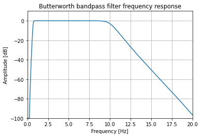
Question: What does this plot tell us about the filter characteristics? What types of noise does the filter attenuate?
Explanation: This function generates the co-efficients for a Butterworth filter. The filter-type is specified as 'bp' - a bandpass filtter. The filter frequencies are specified in Hz (because the sampling frequency, fs, has also been specified): a high-pass frequency of 0.7 Hz, and a low-pass frequency of 10 Hz.
Question: The filter designed here has an order of 10. What would be the impact of reducing the order, to say 4?
Extension 1: How could we re-design the filter to retain frequency content of up to 20 Hz, but eliminate mains frequencies?
Extension 2: What would be appropriate cut-off frequencies when using the PPG for different purposes, e.g. heart rate monitoring, or blood pressure estimation? See this book chapter (Sections 2.2.4 to 2.2.5 on Sampling Frequency and Bandwidth) for details.
Filter the PPG signal
Filter the PPG signal
ppg_filt = sp.sosfiltfilt(sos_ppg, ppg)
Plot original and filtered PPG signals
fig, ax = plt.subplots()
t = np.arange(0, len(ppg_filt))/segment_data.fs

ax.plot(t, ppg,
        linewidth=2.0,
        color = 'blue',
        label = "original PPG")

ax.plot(t, ppg_filt,
        linewidth=2.0,
        color = 'red',
        label = "filtered PPG")

ax.set(xlim=(0, n_seconds_to_load))
plt.xlabel('time (s)')
plt.ylabel('PPG')
plt.xlim([20, 45])

plt.legend()
plt.show()
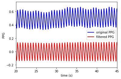
Note: The PPG signals in MIMIC have already been filtered somewhat by the clinical monitors used to record them.
Further work: Several different types of filters have been used to filter the PPG signal (e.g. Chebyshev filter, Butterworth filter). Have a look at this article for examples of several filter types (on pp.8-9). Which type of filter do the authors recommend? Can you re-design the filter above to use this type of filter?
Prepare a segment of clean PPG signal for differentiation
We’ll now extract a segment of clean PPG signal, which we’ll use to show the process of differentiation.
These first few steps are repeated from earlier in this tutorial.
Extract data
Specify the segment
rel_segment_n = 8
rel_segment_name = segment_names[rel_segment_n]
rel_segment_dir = segment_dirs[rel_segment_n]
Load the data for this segment
# Specify the segment of data to be loaded
start_seconds = 100 # time since the start of the segment at which to begin extracting data
n_seconds_to_load = 5

# Load metadata for this record
segment_metadata = wfdb.rdheader(record_name=rel_segment_name, pn_dir=rel_segment_dir)
fs = round(segment_metadata.fs)
print(f"Metadata loaded from segment: {rel_segment_name}")

# Load data from this record
sampfrom = fs*start_seconds
sampto = fs*(start_seconds + n_seconds_to_load)
segment_data = wfdb.rdrecord(record_name=rel_segment_name,
                             sampfrom=sampfrom,
                             sampto=sampto,
                             pn_dir=rel_segment_dir)
print(f"{n_seconds_to_load} seconds of data extracted from: {rel_segment_name}")

# Extract the PPG signal
sig_no = segment_data.sig_name.index('Pleth')
ppg = segment_data.p_signal[:,sig_no]
fs = segment_data.fs
print(f"Extracted the PPG signal from column {sig_no} of the matrix of waveform data.")
Metadata loaded from segment: 88995377_0001
5 seconds of data extracted from: 88995377_0001
Extracted the PPG signal from column 4 of the matrix of waveform data.
Filter this signal segment
Filter the PPG signal
ppg_filt = sp.sosfiltfilt(sos_ppg, ppg)
Plot the signal
Plot the original and the filtered PPG signal
Import the packages required to plot the signal: matplotlib which is used to create plots, and NumPy which is used to create a time vector in this example.
from matplotlib import pyplot as plt
import numpy as np
Make the plot
fig, ax = plt.subplots()
t = np.arange(0, len(ppg_filt)) / segment_data.fs

ax.plot(t, ppg,
        linewidth=2.0,
        label = "original PPG")

ax.plot(t, ppg_filt,
        linewidth=2.0,
        label = "filtered PPG")

plt.xlabel('time (s)')
plt.ylabel('PPG')

plt.legend()
plt.show()
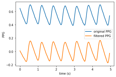
We will use the filtered signal instead of the original PPG from now on.
Differentiate the PPG signal
Differentiate using Savitzky-Golay filtering
Differentiate it once and twice using the Savitzky-Golay filtering function in SciPy
# Calculate first derivative
d1ppg = sp.savgol_filter(ppg_filt, 9, 5, deriv=1)

# Calculate second derivative
d2ppg = sp.savgol_filter(d1ppg, 9, 5, deriv=1)
Resource: Savitzky-Golay filtering, which is used here to calculate derivatives, is described in this article.
Question: Can you summarise how Savitzky-Golay filtering works? What are its advantages in physiological signal processing?
Plot the PPG and its derivatives
t = np.arange(0, len(ppg_filt))/segment_data.fs

fig, (ax1,ax2,ax3) = plt.subplots(3, 1, sharex = True, sharey = False)
ax1.plot(t, ppg_filt)
ax1.set(xlabel = '', ylabel = 'PPG')

plt.suptitle('The PPG signal and its first and second derivatives')

ax2.plot(t, d1ppg)
ax2.set(xlabel = '',
        ylabel = 'PPG\'')

ax3.plot(t, d2ppg)
ax3.set(xlabel = 'Time (s)',
        ylabel = 'PPG\'\'')

plt.show()
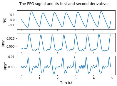
Question: How would the derivatives have looked different if the PPG signal hadn't been filtered before differentiation?
Hint: In the differentiation step above, try replacing 'ppg_filt' with 'ppg'.
Question: How would the derivatives have been different if the PPG signal had been filtered using different co-efficients?
Hint: Above, try replacing the relatively wide band-pass frequencies '[0.7, 10]' with '[0.8, 3]'.
Consider: Which band-pass frequencies would be most suitable for pulse wave analysis? How about heart rate estimation?
Comparison with a typical PPG pulse wave
The figure below shows a typical PPG pulse wave recorded from a young, healthy subject.

Source: Charlton PH, Photoplethysmogram (PPG) pulse wave fiducial points, Wikimedia Commons (CC BY 4.0).
_pulse_wave_fiducial_points.svg)
Question: How does this pulse wave shape and derivatives compare to the shape of those obtained from MIMIC data above? What might explain the differences?
Extension: Try using 'rel_segment_n=3' above (i.e. analysing segment '82439920_0004'). How do the pulse waves in this signal compare? What might that tell us about this patient?
Further reading: this article provides further information on how age affects the shape of the PPG's second derivative.